Were RNNs All We Needed? A GPU Programming Perspective
An implementation of parallelizable GRUs and LSTMs for CS179 in CUDA.
| Resource | Link |
|---|---|
| Project Repository | GitHub |
For my final project in CS179: GPU Programming, I decided to implement the paper “Were RNNs All We Needed?” by Feng et al. The paper’s core claim is that by making minor simplifications to LSTMs and GRUs, their recurrence can be expressed in a form amenable to the parallel scan algorithm. This changes their training and inference from an $O(T)$ sequential process into an $O(\log T)$ parallel one, which helps with GPU acceleration.
My goal was to verify this claim by building both the simplified models (minGRU and minLSTM) and a custom CUDA implementation of the parallel scan to see how much of a speedup was actually achievable. The focus was less on the machine learning application and more on the raw computational performance and the experience of parallelizing a traditionally sequential algorithm.
The Sequential Bottleneck in Standard RNNs
Recurrent Neural Networks, by their very nature, process sequences one step at a time. The hidden state at time step $t$, denoted $h_t$, is a function of the input $x_t$ and the previous hidden state, $h_{t-1}$. This dependency is the fundamental barrier to parallelization.
Let’s look at a standard GRU. The update equations are: \(r_t = \sigma(W_{ir}x_t + b_{ir} + W_{hr}h_{t-1} + b_{hr})\) \(z_t = \sigma(W_{iz}x_t + b_{iz} + W_{hz}h_{t-1} + b_{hz})\) \(n_t = \tanh(W_{in}x_t + b_{in} + r_t \odot (W_{hn}h_{t-1} + b_{hn}))\) \(h_t = (1 - z_t) \odot n_t + z_t \odot h_{t-1}\)
The reset gate ($r_t$) and update gate ($z_t$) both explicitly depend on $h_{t-1}$. You simply cannot compute the gates for the entire sequence in one shot, because each step requires the output from the one before it. This forces a sequential loop, which is notoriously inefficient on parallel hardware like GPUs.
GRU and LSTM –> minGRU and minLSTM
The crux of the paper is to remove this direct dependency. The simplified models, minGRU and minLSTM, redefine the gates to depend only on the current input, $x_t$.
For minGRU, the gates are simplified to:
- Update Gate: $z_t = \sigma(W_z x_t + b_z)$
- Candidate Hidden State: $\tilde{h}_t = W_h x_t + b_h$
The recurrence then becomes: \(h_t = (1 - z_t) \odot h_{t-1} + z_t \odot \tilde{h}_t\)
This equation is now in the form $h_t = a_t \odot h_{t-1} + b_t$, where:
- $a_t = (1 - z_t)$
- $b_t = z_t \odot \tilde{h}_t$
Crucially, because $z_t$ and $\tilde{h}_t$ only depend on $x_t$, we can compute the entire sequence of $(a_t, b_t)$ pairs in parallel with a single, large matrix multiplication. The problem has now shifted from a complex sequential dependency to resolving a linear recurrence relation. A similar simplification is applied to LSTMs to create minLSTM.
The Parallel Scan Algorithm
This linear recurrence is a classic computer science problem that can be solved efficiently with a parallel scan (also known as a prefix sum). The scan operation takes a sequence and an associative binary operator $\oplus$, and computes the prefix results. For our recurrence, the operator is slightly more complex than simple addition.
If we have a transformation $(A, B)$ representing $h_{out} = A \cdot h_{in} + B$, we can define an associative operator $\oplus$ to compose two such transformations: \((A_2, B_2) \oplus (A_1, B_1) = (A_2 A_1, A_2 B_1 + B_2)\)
With this operator, we can use an algorithm like Blelloch’s scan, which performs the computation in two phases (up-sweep and down-sweep) on a tree-like structure. This reduces the number of sequential steps from $O(T)$ to $O(\log T)$, making it a perfect fit for the GPU’s architecture. For numerical stability, the paper and my implementation use a log-space version of this scan.
Implementation & Benchmarking
To measure the real-world impact, I compared three implementation paths:
- CPU-seq: A standard PyTorch loop,
for t in range(T): h_t = cell(x_t, h_{t-1}). This represents the classic, non-parallelizable RNN. - CPU-scan: Computes all gate parameters $(a_t, b_t)$ in one vectorized PyTorch call, but resolves the scan recurrence using a Python loop. This isolates the benefit of vectorization from the parallel scan.
- GPU-scan: My custom CUDA implementation. It uses one kernel to extract all scan parameters and a second kernel to perform the work-efficient Blelloch scan, reducing the recurrence depth to $O(\log T)$.
I ran benchmarks on my personal machine (Intel i9-12900K, RTX 4090).
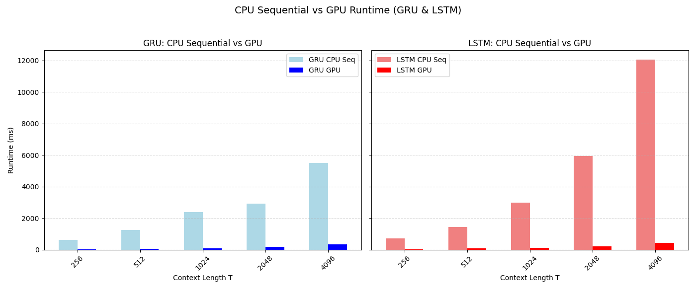
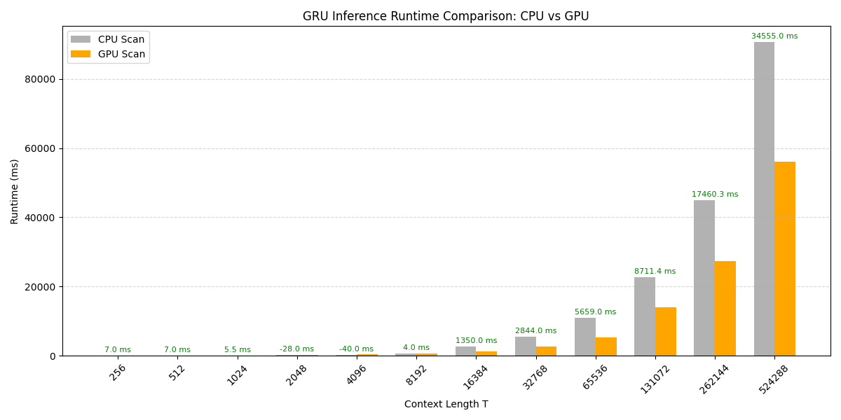
GRU Performance
| $T$ | CPU-seq | CPU-scan | GPU-scan |
|---|---|---|---|
| 256 | 634 ms | 32.8 ms | 25.8 ms |
| 1,024 | 2,395 ms | 97.6 ms | 92.1 ms |
| 4,096 | 5,493 ms | 300 ms | 340 ms |
| 16,384 | – | 2,683 ms | 1,333 ms |
| 65,536 | – | 10,989 ms | 5,330 ms |
LSTM Performance
| T | CPU-seq | CPU-scan | GPU-scan |
|---|---|---|---|
| 256 | 701.0 ms | 37.0 ms | 22.0 ms |
| 1,024 | 2,966.7 ms | 96.8 ms | 107.8 ms |
| 4,096 | 12,035.1 ms | 416.5 ms | 431.5 ms |
| 16,384 | – | 2,993.6 ms | 1,693.9 ms |
| 65,536 | – | 13,005.4 ms | 6,709.8 ms |
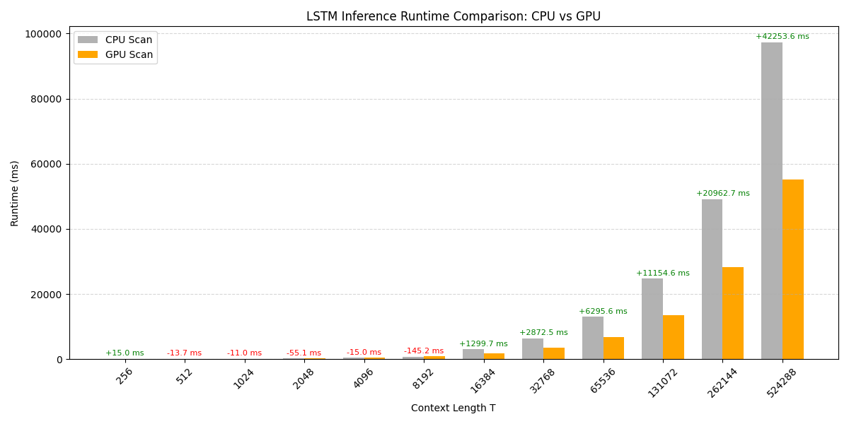
Observations:
- For short sequences ($T < 2048$), the overhead of launching CUDA kernels and memory transfers negates some of the benefits of the parallel scan. The CPU-scan implementation, which benefits from highly optimized BLAS libraries (like MKL), is sometimes faster.
- For long sequences ($T > 8192$), the algorithmic advantage of the $O(\log T)$ GPU scan becomes dominant. At $T=65,536$, the GPU implementation is roughly 2x faster than the vectorized CPU version and would be orders of magnitude faster than the purely sequential version.
- Vectorizing the gate computations alone (
CPU-seqvsCPU-scan) provides a massive, constant-factor speedup (around 10x), but the runtime still scales linearly, $O(T)$.
GPU Kernel Profiling with Nsight
To understand the GPU performance better, I used NVIDIA’s Nsight Compute profiler. The initial implementation launched thousands of tiny kernels, one for each time step, which is a classic anti-pattern in GPU programming due to launch overhead.
My first major optimization was to fuse the gate computations for all time steps into a single, large kernel (min_gru_extract_scan_params_kernel) that uses shared memory tiling to manage weights and inputs efficiently.
Here’s a snapshot of the kernel performance breakdown at $T=4096$ after this optimization:
| Rank | Kernel | Time/launch | Launches | % wall-time |
|---|---|---|---|---|
| 1 | min_gru_extract_scan_params_kernel | 180 $\mu$s | 1 | 8 % |
| 2–9 | compose_offset_kernel (Scan Up-Sweep) | ~3 $\mu$s | 12 | < 1 % |
| 10– | apply_scan_op_kernel (Scan Down-Sweep) | ~2 $\mu$s | 4096 | 10 % |
| 11– | matvec_kernel (Output Projection) | ~93 $\mu$s | 4096 | 72 % |
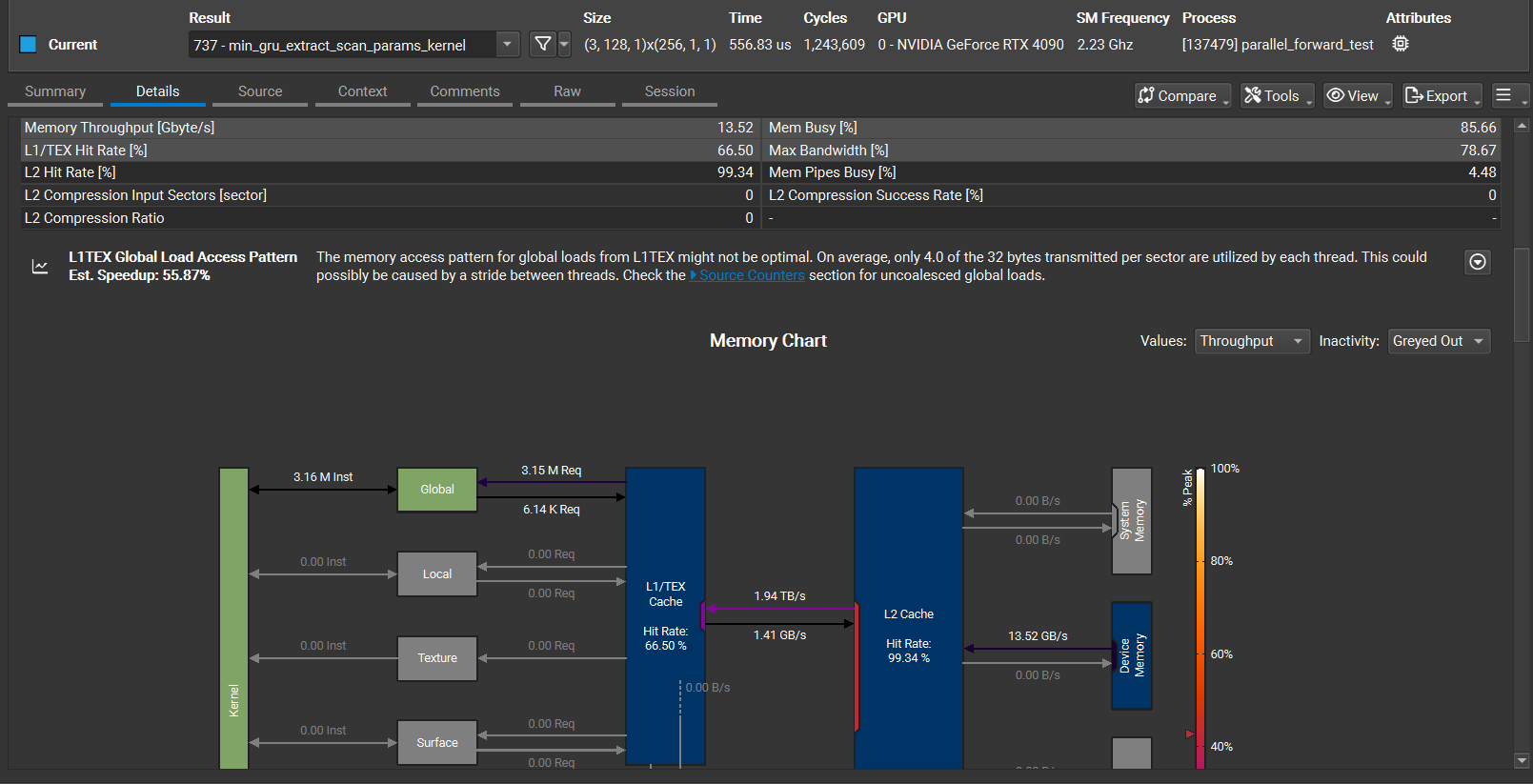
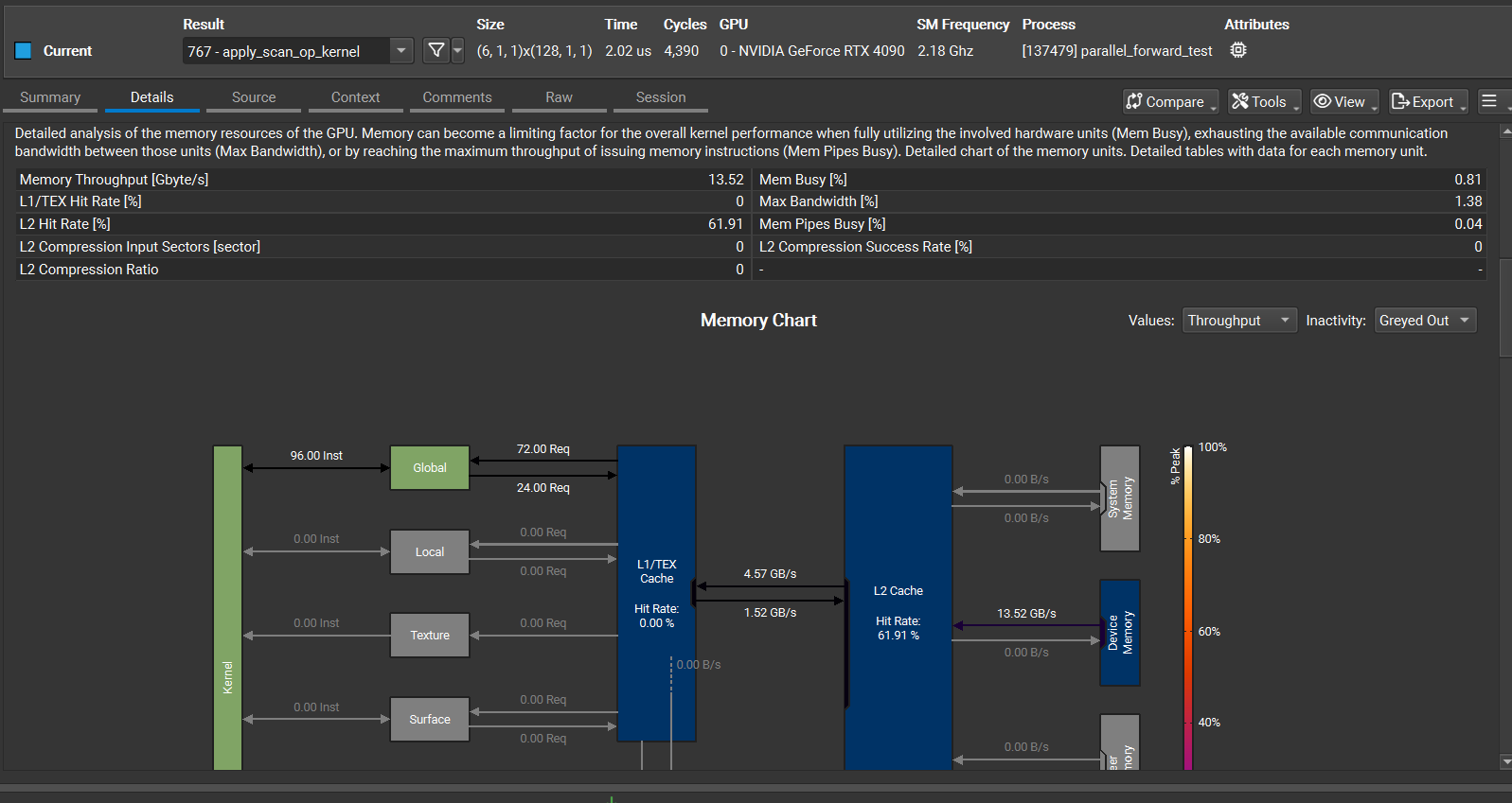
The profiling revealed a few things:
- Success: The gate extraction kernel, which was a huge bottleneck, now only takes 8% of the total time and is memory-bandwidth bound, saturating L2 bandwidth at 1.9 TB/s. This is a good place to be.
- New Bottleneck: The primary bottleneck shifted to the final projection layer (
matvec_kernel), which consumes 72% of the runtime. This is because I was still launching one kernel per time step (4096 launches!), leading to low occupancy and terrible memory bandwidth utilization (only 23 GB/s). - Next Step: The next step is to replace the 4096
matveclaunches with a single cuBLAS GEMM call ($C = A \cdot W^T$). This would eliminate the kernel launch overhead and leverage a highly optimized library routine, likely bringing the total latency down significantly.
Final Thoughts
I made this project as part of my final assignment for my GPU Programming course, CS 179 at Caltech. This project was a great hands-on lesson in parallel algorithms. The claims in “Were RNNs All We Needed?” did seem to hold up: by reformulating the recurrence, RNNs can indeed be parallelized, and the performance gains on GPUs are substantial for long sequences. One of the reasons why this paper gained criticism from the CS commmunity was because there weren’t many experiments to back the claim that miniRNNs performed any better than transformers - and from my rusty recollection of the paper - the only benchmarks the miniRNNs outperformed transformers were niche targetted datasets that did not transfer to real-world benchmarks. Sure, with the parallelization and ripping away unncessary complexity from RNNs, miniRNNs were much more efficient but it was never the end-all be-all.
I remember Francois’s quote on this paper from his X thread:
Interesting work on reviving RNNs. https://arxiv.org/abs/2410.01201 – in general the fact that there are many recent architectures coming from different directions that roughly match Transformers is proof that architectures aren’t fundamentally important in the curve-fitting paradigm (aka deep learning)
Curve-fitting is about embedding a dataset on a curve. The critical factor is the dataset, not the specific hard-coded bells and whistles that constrain the curve’s shape. As long as your curve is sufficiently expressive all architectures will converge to the same performance in the large-data regime.
I have a different take on this. All progress in the language modelling in the last decade has come from changes in architectures to be able to generate rich, more expressive curves that fit the target dataset better. If we blindly apply the bitter lesson and throw enough compute to different architectures (reasonable ones), it would be a good signal to see which architecture hits the wall the fastest and which one continues generalizing rather than all converging in the same way eventually.